YOLOv8 on Salad
Introduction
Object detection technology has come a long way from its inception. Early systems could hardly differentiate between shapes, but today’s algorithms like YOLOv8 have the ability to pinpoint and track objects with remarkable precision. YOLOv8 is the latest advancement in a lineage known for balancing accuracy and speed. Unlike the AI of old that would chug through data, YOLOv8 skates across live feeds, identifying and classifying objects with an efficiency that supports a multitude of practical applications. It could be tracking logos screen presence during sporting event, monitoring items on an assembly line, or inspecting the intricate parts of train cars for maintenance. YOLOv8 offers a lens through which the world can be quantified in motion, without the need for extensive model training from the end user. Deploying YOLOv8 on SaladCloud results in a practical and efficient solution. SaladCloud’s infrastructure democratizes the power of YOLOv8, allowing users to deploy sophisticated object detection systems without heavy investment in physical hardware. Whether you’re a developer or a business looking to integrate cutting-edge object detection into your operations, YOLOv8 paired with SaladCloud offers a viable and scalable solution. Stay tuned as we dive into creating our object detection solution with Yolov8 within the environment of SaladCloud , showcasing how this combination can streamline your object detection needs.Project Overview: Streamlining Object Detection in Live Streams with YOLOv8 and SaladCloud
In this project, we focus on harnessing the power of a pre-trained YOLOv8 model to analyze live video streams. In this article, we will not delve into training our custom model, but it may be an avenue we explore later. The Workflow:- Input Data: We initiate the process by capturing a live stream link as our input source. This will be live stream video upon which object detection will be performed.
- Object Detection: With each passing frame of the live video, YOLOv8’s pre-trained algorithms analyzes the visuals to detect objects it has been trained to recognize.
- Data Compilation and Analysis: As objects are identified, their information is systematically captured in real time, leading to the construction of a comprehensive dataframe. This tabular data encompasses timestamps, object classifications, and other pertinent metadata extracted from the video frames. Utilizing aggregation methods and analytical techniques, we’ll further refine this data to create a concise and informative summary.
- Storage and Accessibility: The dataframe is then exported as a CSV file, which is securely stored in an Azure storage account. This ensures easy access and manageability of the processed data for further analysis or record-keeping.
- Human-Friendly Summaries: Beyond the raw data, we gather information into human-readable summaries. These narratives will provide insights into how long specific objects were present in the video and what percentage of the frame the were taking.
- No Need for Model Training: We can use a pretrained Yolo Model for our demo saving some time on data labeling and training. We might cover training in one of our next articles.
- Real-Time Analysis: Processing live streams requires potent computational resources. Deploying our solution on SaladCloud offers the necessary horsepower without the overhead of local infrastructure.
- Data-Driven Insights: Our approach converts continuous video streams into structured data, paving the way for in-depth analytics and informed decision-making.
- Accessible Results: By storing outcomes in Azure, we benefit from cloud scalability and the robustness of enterprise-grade security and data handling.
- Comprehensive Reporting: The human-friendly summaries bridge the gap between complex data analytics and actionable insights, useful for non-technical stakeholders.
Reference Architecture
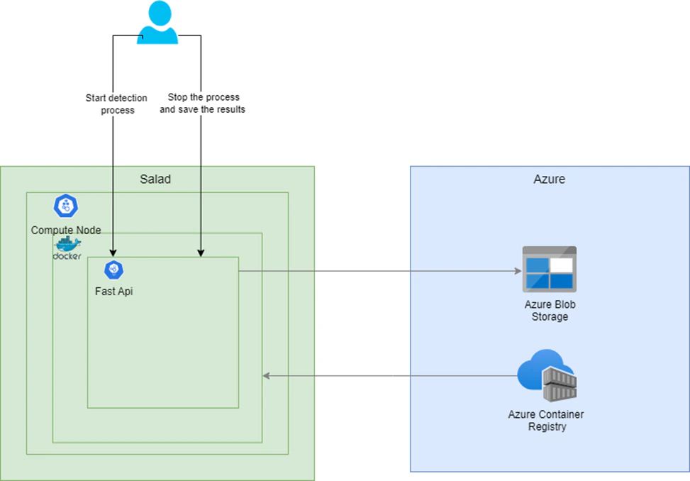
We are setting out to construct two distinct solutions to leverage the capabilities of YOLOv8 for object detection. Here’s an outline of the architecture for each solution:Solution 1: Fast API for Real-Time Processing
- Objective: Develop an API that can initiate and terminate the object detection process based on API calls.
- Process Flow:
- The Fast API receives a request with all the necessary parameters to start the object detection task.
- It processes the video stream in the background, identifying and classifying objects as they appear.
- Upon receiving a stop API call, the process concludes, and the results are stored in an Azure storage container.
- Deployment:
- The Fast API is containerized using Docker, ensuring a consistent and isolated environment for deployment.
- This Docker container is then deployed on SaladCloud compute resources to utilize processing capabilities.
- The Docker image itself is housed in Azure Container Registry for secure and convenient access.
Solution 2: Batch Processing for Asynchronous Workloads
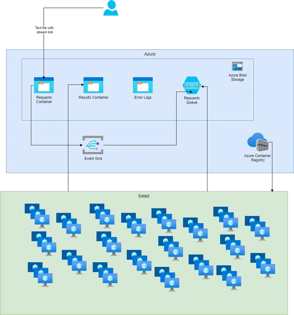
- Objective: Set up a batch processing system that reacts to new video stream links stored in Azure.
- Process Flow:
- Video stream links are saved in an Azure storage container.
- An event grid with subscriptions is configured to monitor the storage container and trigger a message in a storage queue whenever a new file is added.
- A Python script for batch processing is containerized and deployed across multiple SaladCloud compute nodes.
- This batch process routinely checks the storage queue. When a new message appears, it picks up the corresponding stream for processing.
Folder Structure
Our full solution is stored here: git repo Here is the folder structure we will have once the project is done:Local Environment Testing
Before we deploy these solutions on SaladCloud’s infrastructure, it’s crucial to evaluate YOLOv8’s capabilities in a local setting. This allows us to troubleshoot any issues and make any make our solution meet our needs.Local Development Setup: Installing Necessary Libraries
Setting up an efficient local development environment is essential for a smooth workflow. I ensure this by preparing setup and requirements files to facilitate the installation of all dependencies. These files help verify that the dependencies function correctly during the development phase. I am providing the complete contents of the requirements file and the setup script above. During my work on the project, I encountered a couple of issues with the libraries, which I will briefly mention without going too deeply into them.Encountered Issues and Their Workarounds:
Issue 1: Processing YouTube Videos and Live Streams The library ‘pafy’ is commonly used to process YouTube video URLs and is dependent on ‘youtube-dl’, which hasn’t been updated recently. YouTube’s API change, specifically the removal of the dislike count, has led to ‘youtube-dl’ encountering errors regarding the ‘dislike_count not found’. To circumvent this, I’ve switched to using the ‘cap_from_youtube’ library, which is a simplified alternative to ‘pafy’. It simply retrieves the video URL and creates an OpenCV video capture object. Issue 2: Module Not Found Error in Virtual Environment Utilizing Yolo tracking within a Python virtual environment was throwing a “ModuleNotFoundError: No module named ‘lap’”. Attempting to resolve this issue led me down a rabbit hole of dependency ordering, specifically the need to install ‘numpy’ before ‘lap’. The only effective solution was to downgrade ‘pip’, install ‘lap’, upgrade ‘pip’ again, and then proceed with installing the remaining requirements. This installation sequence has been replicated in the Dockerfile as well. The Setup Script:Python
Bash
Exploring YOLOv8’s Capabilities and Data Compatibility
As we delve into the practicalities of implementing YOLOv8 for object detection, a fundamental step is to understand the range of its capabilities and the types of data it can process effectively. This knowledge will shape our approach to solving the problem at hand. Here is a list of possible inputs: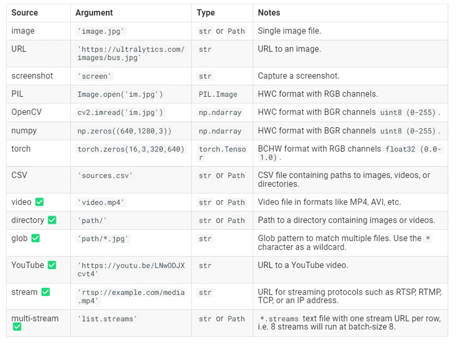
Video processing
We’ll begin by experimenting with an example straight from the Ultralytics documentation, which illustrates how to apply the basic object detection model provided by YOLO on video sources. This example uses the ‘yolov8n’ model, which is the YOLOv8 Nano model known for its speed and efficiency. Here’s the starting code snippet provided by Ultralytics for running inference on a video: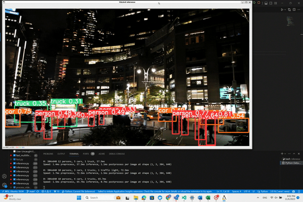
Processing Live Video Stream from Youtube
Now we move on to the task of processing live video streams. While cap_from_youtube works well for YouTube videos by loading them into memory, live streams require a different approach due to their continuous and unbounded nature. Pafy is a Python library that interfaces with YouTube content, providing various streams and metadata around YouTube videos and playlists. To make it work in the virtual environment we had to solve a few libraries issues we discussed earlier. To make the process easier for you run the dev/setup file we also mentioned earlier. For live video streams, Pafy allows us to access the stream URL, which we can then pass to OpenCV for real-time processing. Here’s how we can use Pafy to open a live YouTube stream:Processing Live Video Stream (RTSP, RTMP, TCP, IP address)
Ultralytics gives us an example of running inference on remote streaming sources using RTSP, RTMP, TCP and IP address protocols. If multiple streams are provided in a*.streams text file then batched inference will run, i.e. 8 streams
will run at batch-size 8, otherwise single streams will run at batch-size 1. We will include it in our code as well.
Based on specific link parameters our process will pick which way to process the link. You can check that in the full
script
Implementing Object Tracking
Having established the method to process live streams, the next crucial feature of our project is to track the identified objects. YOLOv8 comes equipped with a built-in tracking system that assigns unique IDs to each detected object, enabling us to follow their movement across frames. There is a way to pick between 2 tracking models, but for now we will just use the default one. Enabling Tracking with YOLOv8: To utilize the tracking functionality, we simply need to modify our inference call. By adding .track to our model call and setting persist=True, we instruct the model to maintain object identities consistently over time. This addition to the code will look like this: That is great, but our main goal is to get a summary of how long an object was present on the video. I will now remove
the appearing window with the bounding boxes and we will pay more attention to the data. For this part of the project I
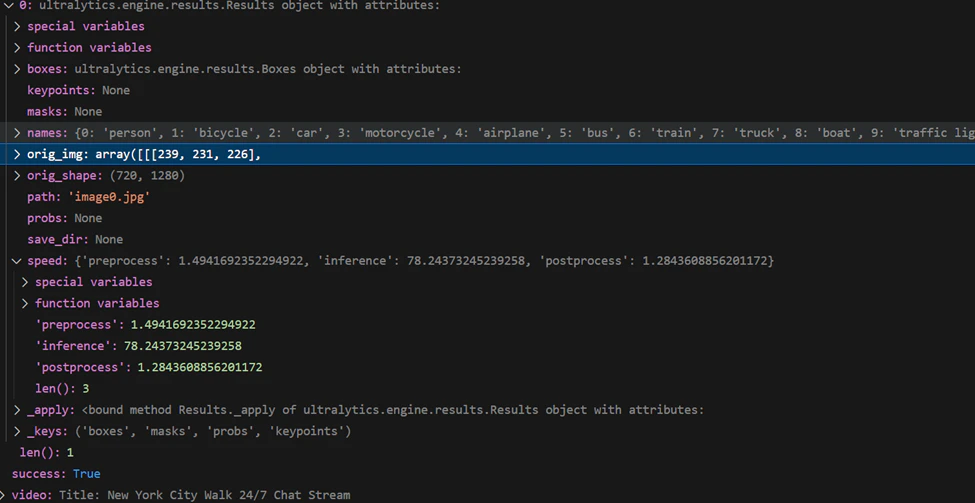
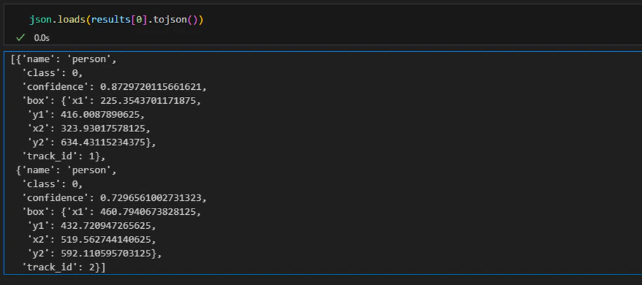
am using Jupyter in vscode and pandas. Let’s check what results object is:
That is great, but our main goal is to get a summary of how long an object was present on the video. I will now remove
the appearing window with the bounding boxes and we will pay more attention to the data. For this part of the project I
am using Jupyter in vscode and pandas. Let’s check what results object is:
Readable summary
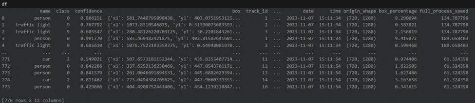
With the DataFrame populated with tracking and detection data, we’re now ready to create a summary that achieves our main goal: calculating the duration each object was present in the video. We’ll start by filtering out any irrelevant data and then proceed to group the valid detections to summarize our findings. Filter data We need to ensure that we only include rows with valid tracking IDs. This means filtering out any detections that do not have a tracking ID or where the tracking ID is 0, which may indicate an invalid detection or an object that wasn’t tracked consistently. Grouping Detections for Summary: With a DataFrame of filtered results, we’ll group the data by tracking ID to find the earliest and latest timestamps for each object. Our object will get a new tracking ID if it leaves and re-enters the video. If in your project you need to track a specific label, you will need to add additional logic of grouping by class and summing the durations. We’ll also determine the most commonly assigned class for each object, in case there are discrepancies in classification across frames, and calculate the average size of the object within the frame. The summary function will perform these operations and output a readable string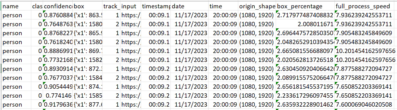
Storing Object Detection Results in Azure Storage
Create Storage Account Storing your YOLOv8 object detection results in Azure Storage is an excellent way to manage and archive your data efficiently. In order to be able to do that we created an account in Azure, created a subscription, resources group, storage account and a storage container name “yolo-results“. Since we only needed a storage account for our api solution we provisioned in through the portal. For our “batch“ process we created a bicep file that you can check here. You can find a very detailed documentation on how to create a storage account from Microsoft here Next we got our storage connection string. To do that open azure portal and navigate to your storage account. On the left click “Access keys“. Click “show“ next to Connection string and save it somewhere. Here is a little function we put together to connect to our storage account that uses container name and storage key as inputs:- Timed Saves: We implement logic within the processing loop to save interim results at intervals that will be specified in our api call. Since our stream might be infinite we need to do to be able to check the results without breaking the connection to the stream.
- Final Save: Ensure all results are saved once the process is completed:
Create FastAPI
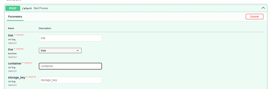
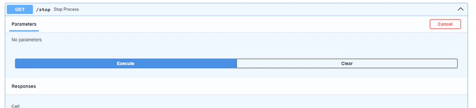
We have verified that our yolo model does it’s job, we’ve put together the logic of saving our results and configured our azure storage account. Now let’s pack and deploy our solution to cloud. Among various options, we’ve opted for an API-based approach and chosen Python FastAPI for several compelling reasons. FastAPI stands out for its high performance and efficient asynchronous support, essential for handling our real-time data processing demands. Additionally, it offers the convenience of automatic interactive documentation with a prebuilt Swagger interface, simplifying the use and understanding of our API. We ill create 3 api endpoints: Start Endpoint: An endpoint to initiate the object detection process as a background task. It accepts parameters like link, live, container, saving timer and storage_key necessary for the process. Stop Endpoint: An endpoint to halt the ongoing object detection process. It sets a global flag should_continue to False to signal the process to stop. Health Check Endpoint: A simple endpoint to check the health of the service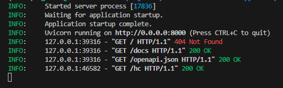

Containerizing the FastAPI Application with Docker
Now that we have our FastAPI tested and verified, the next crucial step is to package our solution into a Docker image. This approach is key to facilitating deployment to our cloud clusters. Containerizing with Docker not only streamlines the deployment process but also ensures that our application runs reliably and consistently in the cloud environment, mirroring the conditions under which it was developed and tested. With Docker, we create a portable and scalable solution, ready to be deployed efficiently across various cloud infrastructures. When creating the Dockerfile, it’s crucial to select a base image that includes all the necessary system dependencies, because that might cause some networking issues. We’ve tested our solution with “python3.9“ base image, so if possible stick to it. If you have to use a different base image for any reason check out SaladCloud documentation on networking. We should also keep in mind our earlier issues with the libraries. Here is the full Dockerfile we will use to build an image:Deploying the FastAPI Application to Salad
We finally got to the last and most exiting part of our project. We will now deploy our full solution to the cloud. Deploying your containerized FastAPI application to SaladCloud’s GPU Cloud can is a very efficient and cost-effective way to run your object detection solution. SaladCloud’s has a very user-friendly interface as well as an API for deployment. Let’s deploy our solution using SaladCloud portal. First create your account and log into the portal Create your organization and let’s deploy our container app. Under Custom Container Group click “Get Started”: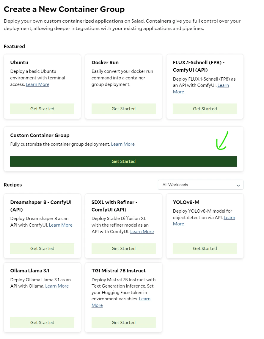
- Create a unique name for your Container group
-
Pick the Image Source: In our case we are using a private Azure Container Registry. Click Edit next to Image
source. Now switch to “Private Registry“, under “What Service Are You Using“ pick Azure Container Registry. Now lets
get back to our azure portal and find the image name, username and password of our container registry repository.
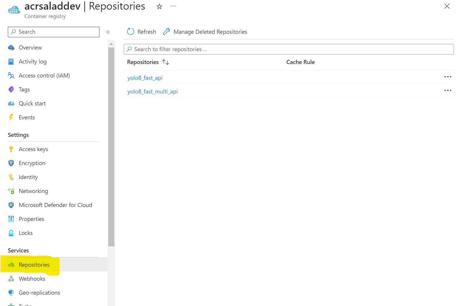
Find your acr in azure and click “repositories“ on the left
docker pull <image name>: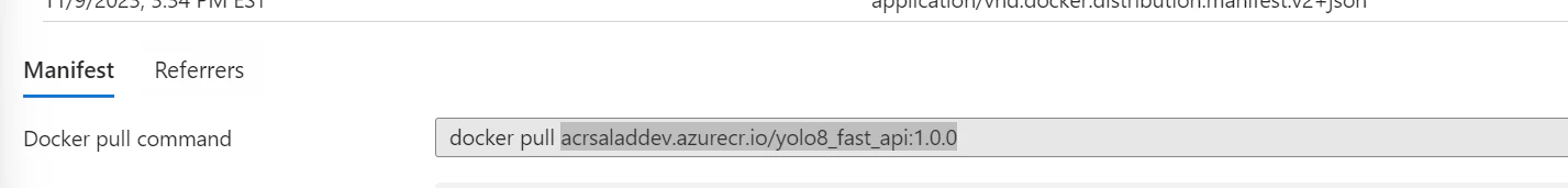
- Replica count: I will pick for now, since our process is kind of “synchronous“. We will use the second replica as a backup.
- Pick compute resources: That is the best part. Pick how much cpu, ram and gpu you want to allocate to your process. The prices are very low in comparison to all the other cloud solutions, so be creative.
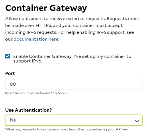
- Optional Settings: SaladCloud gives you some pretty cool options like health check probe, external logging and passing environment variables. For our solution the one parameter that we have to pass is the Container Gateway. Click “Edit“ next to it, check “Enable Container Gateway“ and set port to 80:
Benefits of Using Salad:
- Cost-Effectiveness: SaladCloud offers GPU cloud solutions at a more affordable rate than many other cloud providers, allowing you to allocate more resources to your application for less.
- Ease of Use: With a focus on user experience, SaladCloud’s interface is designed to be intuitive, removing the complexity from deploying and managing cloud-based applications.
- Documentation and Support: SaladCloud provides detailed documentation to assist with deployment, configuration, and troubleshooting, backed by a support team to help you when needed.
Test Full Solution deployed to Salad
With your solution deployed on Salad, the next step is to interact with your FastAPI application using its public endpoint. SaladCloud provides you with a deployment URL, which you can use to send requests to your API in the same way you would locally, but now through SaladCloud’s infrastructure.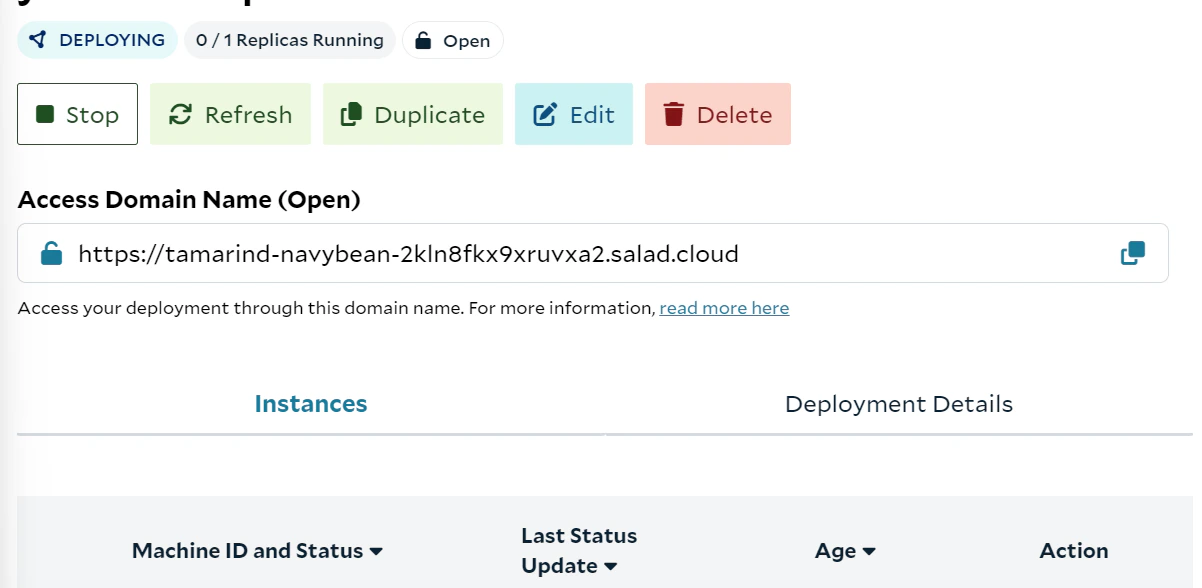

Price Comparison: Processing Live Streams and Videos on Azure and Salad
When it comes to deploying object detection models, especially for tasks like processing live streams and videos, understanding the cost implications of different cloud services is crucial. Our comparison will consider three scenarios: processing a live stream, a complete video, and multiple live streams simultaneously. Let’s start with the first use case: live streamContext and Considerations
- Live Stream Processing: Live streams are unique in that they can only be processed as the data is received. Even with the best GPUs, the processing is limited to the current feed rate.
- Azure’s Real-Time Endpoint: We assume the use of an ML Studio real-time endpoint in Azure for a fair comparison. This setup aligns with a synchronous process that doesn’t require a full dedicated VM.
Azure Pricing Overview
We will now compare the compute prices in Azure and SaladCloud. Note that in Azure you can not pick ram, vCpu and GPU memory separately. You can only pick preconfigured computes. With SaladCloud you can pick exactly what you need.- Lowest GPU Compute in Azure: For our price comparison, we’ll start by looking at Azure’s lowest GPU compute price, keeping in mind the closest model to our solution is YOLOv5.
1. Processing a Live Stream
Percentage Cost Difference for General Compute
- SaladCloud is approximately 83% cheaper than Azure for general compute configurations.
2. Processing with GPU Support. This is the GPU Azure recommends for YOLOv5.
Percentage Cost Difference for GPU Compute
- SaladCloud is approximately 73% cheaper than Azure for similar GPU configurations.